Adding Your Own Geospatial Data to Your Workspace

UNBL workspaces support the upload of geospatial raster data in the following file format:

• GeoTIFF (Georeferenced Tagged Image File Format)

UNBL workspaces also support the connection to external geospatial data through any of the following external tile service providers:

• WMS (Web Map Service)

• WMTS (Web Map Tile Service)

• Google Earth Engine (GEE)

• Spatiotemporal Asset Catalog (STAC) (not ready yet - coming soon!)

• XYZ Tile Service

• Mapbox

• ESRI ArcGIS API Map Service through WMS, WMTS, or vector tile service

• Vector Tile Services (served as pg_tileserv or Martin)

Geospatial data can be uploaded and/or linked to within your workspace, thereby giving all your workspace members the ability to view your data on UNBL without them needing any prior GIS experience. UNBL security ensures that datasets within your workspace are only visible to members of your workspace. However, if you want datasets within your workspace to be viewable by anyone outside of your workspace, you can enable this using a public layer URL option. Only people with access to this URL will be able to view your layer. For further details around data privacy, please see our overview sheet on data security.

Importantly, any datasets in your workspace can also be viewed in tandem with global datasets published on UNBL’s public platform.

Note

The terms dataset and layer are used intermittently henceforth. A dataset refers to a collection of spatial data consisting of one or more layers. On UNBL, a single upload or configuration of geospatial data is realized through ‘creating a layer’. Multiple layer entries can be combined and visualized on UNBL as a dataset. Single layers can also be visualized independently on UNBL.

What parameters and metadata do I fill in when creating a layer?

To begin creating a layer and fill in relevant metadata for the layer:

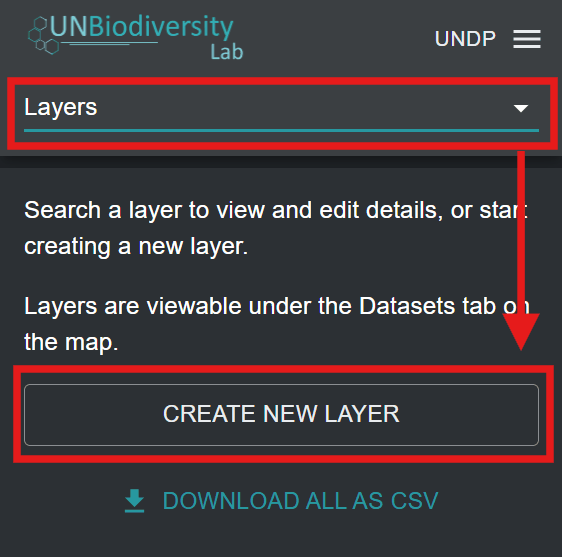
1. Open the ‘Home’ dropdown menu in your workspace admin interface and click on ‘Layers’.

2. Click the ‘CREATE NEW LAYER’ button.

   

   Figure 1: Layers selected in the admin dropdown menu with the CREATE NEW LAYER button highlighted

3. In the new layer page, fill in the following information:

   a. Layer title: The name of your layer. This should be concise (we recommend that it is less than 100 characters in length) and descriptive of your data.

   b. Layer slug: A slug is a unique identifier for the layer within your workspace. You cannot have multiple layers within your workspace with the same slug. It should contain only letters, digits, and hyphens (“-”). You can use the ‘GENERATE SLUG NAME’ button to generate a unique identifier based on the supplied layer title.

   c. Layer category (optional): You can select one or more categories for the layer from the list of options in the dropdown menu. A wide range of socioeconomic, nature-based, and KMGBF policy-related categories are available. More than one category can be selected for the same layer. These categories correspond to the dataset category filters in the map view. Selecting a category will mean that your layer will appear in the list of filtered datasets when the corresponding dataset category filter is applied.

   d. Tag (optional): You can specify one or more tags for your layer. Tags correspond to the dataset tags filter in the map view. Specifying a tag for your layer will mean that the layer will appear in the list of filtered layers when the corresponding dataset tag filter is applied in the map. Unlike layer categories, tags can be any text string of your choice, making this feature useful if you need to clearly differentiate your workspace layers from public platform datasets and be able to apply more effective filters when searching for your datasets in the map view. For example, you could use a tag to identify the target in your national biodiversity strategy and action plan (NBSAP) for which the data layer is relevant.

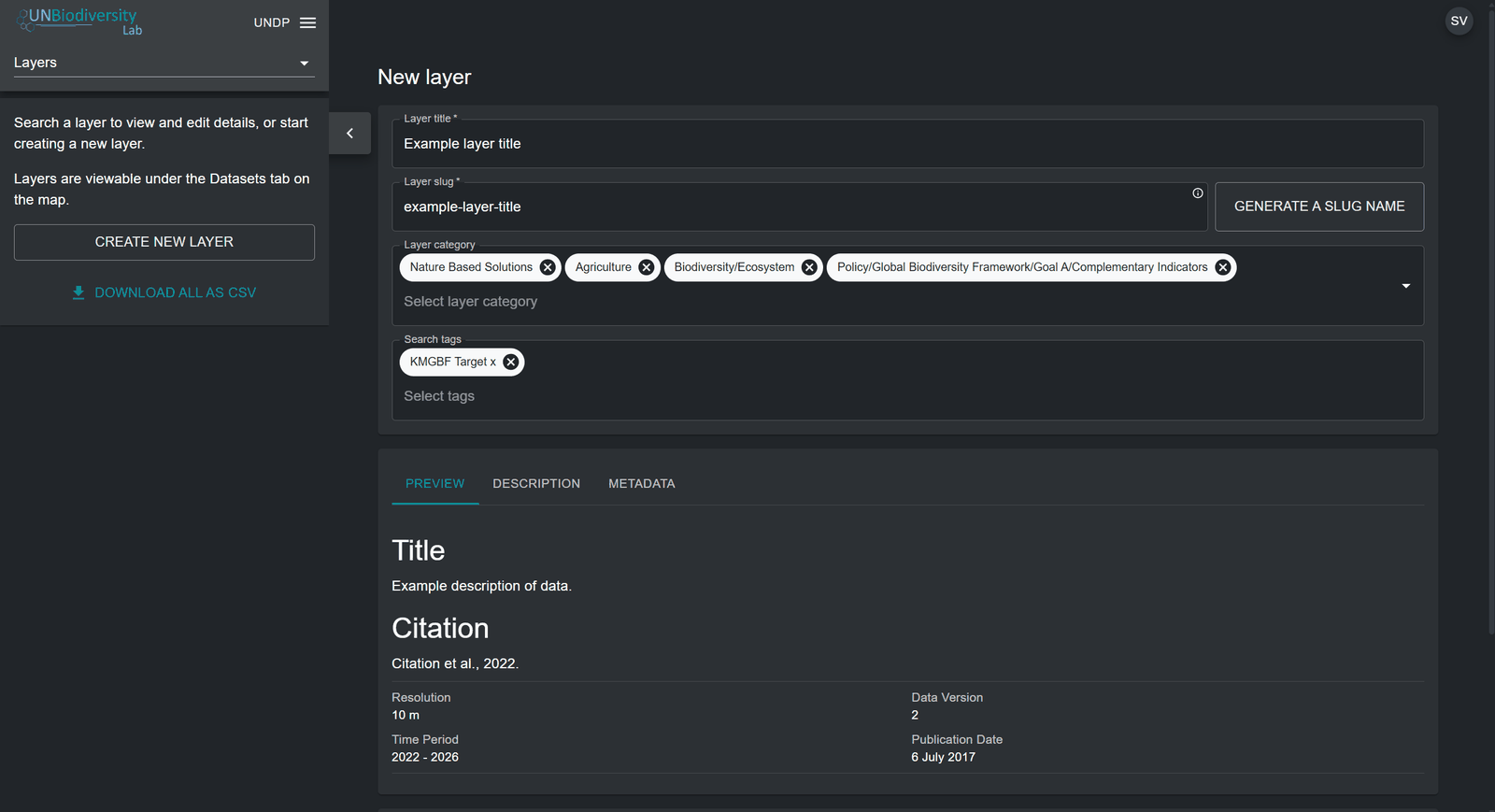
   e. Layer description (optional): In the description field, you can specify the text that will appear in the layer information pop-up box. Here, you can insert the bulk of your layer metadata, such as a general description, citation for the scientific paper/dataset, external links to the scientific paper/dataset, licence specifications, etc. There is an additional 'METADATA' parameter which permits you to fill in concrete data parameters such as the resolution, data version, dataset date and publication date. The 'PREVIEW' parameter allows you to preview how the layer information pop-up box will look like on UNBL.

   Note

   For layers that are part of a group layer, the layer information pop-up shows the group layer's description first, followed by the layer's own description. Use the group layer's description for information that applies to all of its layers, and the layer's own description only for what is specific to that layer (see ‘How do I create group layers?’).

   

   Figure 2: New layer page with title, slug, categories, search tags and description preview filled in

4. Once you have filled in the relevant metadata to document this new layer, you now need to specify the format or geospatial web service standard of your geospatial data and set up the layer configuration accordingly. The forthcoming sections detail how to configure your layer based on the format of your geospatial data.

How do I upload raster layers in GeoTIFF format?

Currently, you can manually upload geospatial data to your UNBL workspace only if it is available in a raster GeoTIFF format. A raster layer constitutes a grid of cells (or pixels) where each cell has a value representing information about a specific topic or phenomenon. We can currently accept only GeoTIFFs with one single band. If you have a GeoTIFF with more than one band, split it upfront into different files. GeoTIFF raster layers are added to your UNBL workspace through a direct upload to a secure, GDPR-compliant UNBL GIS data repository on Azure. For further information, please see our overview sheet on data security.

Note

Geospatial data in other raster and vector layer formats can be configured on UNBL through linking to an external resource. See ‘How do I configure raster layers using external tile services?’ and ‘How do I configure vector layers using external tile services?’ for available UNBL-interoperable OGC Web Service formats and guides on linking to them.

To upload a GeoTIFF file:

1. Navigate to the new layer page and fill in relevant metadata (See ‘What parameters and metadata do I fill in when creating a layer?’).

2. In the 'Layer Config' section:

   a. Layer type: Select ‘raster’.

   b. Layer provider: Select ‘GeoTIFF File Upload’.

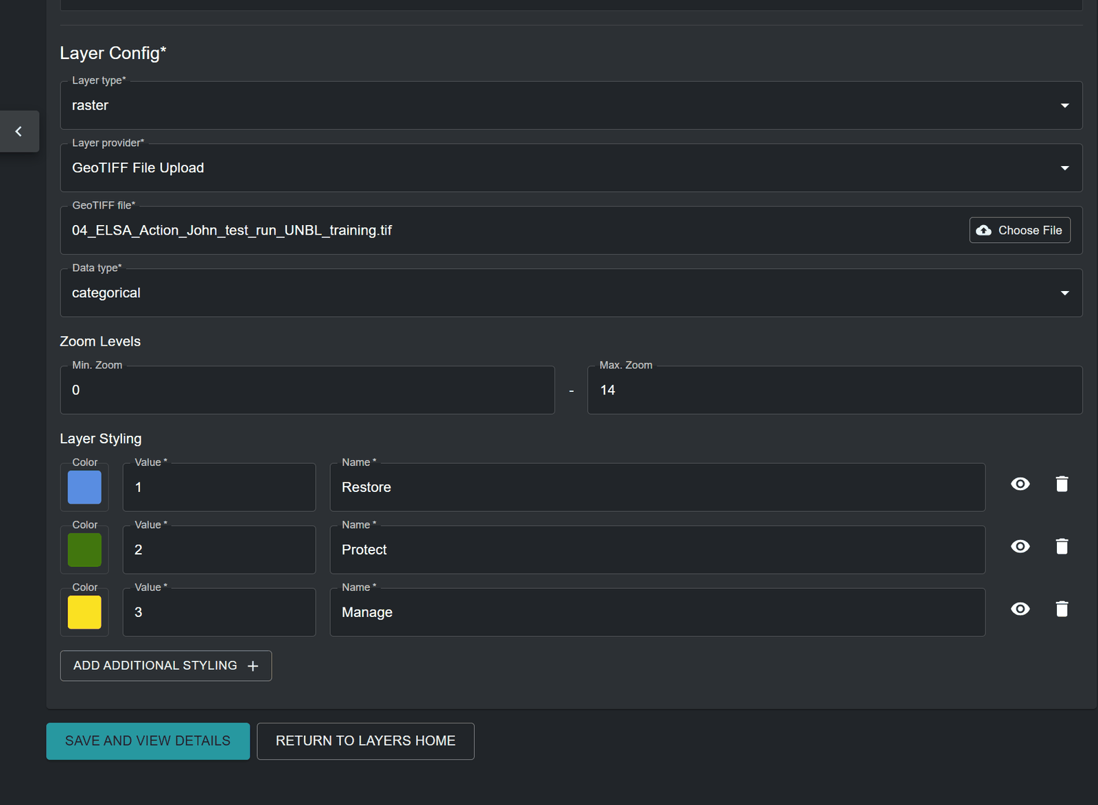
   c. GeoTIFF file: Click the ‘Choose File’ button to upload a valid GeoTIFF raster layer from your local file system. Uploaded files should be a single-band raster and should be less than 1000MB in size. You will be notified if you select an invalid file.

   d. Data type: Specify whether the raster contains ‘categorical’ or ‘continuous’ data. Categorical data represents discrete classes or categories where each pixel value represents a distinct type or class (for instance, Land Use Land Cover classes). Continuous datasets represent data where values can fall anywhere within a specified range of values (for instance, yearly mean temperature).

   e. Minimum/Maximum value: If your raster contains continuous data, then you must supply the range of values in the data by specifying minimum and maximum values of the range.

   f. Minimum/Maximum zoom level (optional): The default zoom level range is set to 0 to 14. You can optionally specify the zoom levels for the layer if the raster file only contains data at certain zoom levels. Note that UNBL supports a maximum zoom level of 14.

   g. Layer styling: The layer styling determines how the layer is displayed on the map. By clicking on ‘ADD ADDITIONAL STYLING’ you can specify any number of layer styling entries to match the values in your raster. Each layer styling entry should define the following properties:

   • Value - the pixel value in the data to define the styling for.

   • Name – the name of the styling entry in the layer legend on the map.

   • Color – the colour of pixels with the specified value on the map. You can define a colour through the manual colour picker, or by entering a RGBA or Hexadecimal value. Optionally, you can set the opacity of the colour in a range from 0 to 100%, where 0% is fully transparent and 100% is fully opaque.

   You can also optionally choose whether a styling entry’s name label is hidden in the layer legend on the map by clicking the

   icon next to the styling entry. For categorical layers, layer styling value entries must map to the values of each category/class within the raster data source. For continuous layers, layer styling value entries must map to the range of values within your raster file that you want rendered on the map. You can specify any points along the range of values between the minimum and maximum values -- a gradient of colours between each of these values will be generated.

   Figure 3: Visibility toggle (eye)

   

   Figure 4: Layer configuration for a GeoTIFF File Upload with three categorical layer styling entries

3. Once all metadata and parameters have been specified, the ‘SAVE AND VIEW DETAILS’ button will light up blue, provided that all the entered information is valid. Click on this button to upload your GeoTIFF file to your workspace. The file will be stored in a safe and dedicated private repository on Azure. This may take a few seconds depending on the size of the file and the speed of your upload internet broadband, so after clicking the button you should wait until you are redirected to the edit layer page. See ‘How do I publish my layer and share it with external users?’ and ‘How do I edit my added layers?’ for next steps.

How do I configure raster layers using WMS/WMTS external tile services?

UNBL supports the configuration of raster image layers to your workspace by linking to external tile service providers. To add geospatial data to your workspace using this method:

1. Navigate to the new layer page and fill in relevant metadata (See ‘What parameters and metadata do I fill in when creating a layer?’).

2. In the 'Layer Config' section:

   a. Layer type: Select ‘raster’.

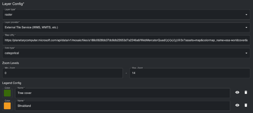
   b. Layer provider: Select ‘External Tile Service (WMS, WMTS, etc.)’.

   c. Tiles URL: Here, you can connect to an external tile service that uses the Web Map Service (WMS), Web Map Tile Service (WMTS), or XYZ Tile Service protocols. To configure layers using these providers, you must supply a valid tile URL, which must contain either the placeholders {z}{x}{y} or the placeholder {bbox-epsg-3857}.

   For example, the sample WMS URL below will not work:

   https://wms.server.net/mapserv?request=getmap&service=wms&BBOX=-90,-180,90,360&crs=EPSG:4326&format=image/jpeg&layers=layer_latest&width=1200&height=600
   

   as it contains an incorrect bounding box (BBOX) parameter format. The URL can be adjusted by changing the BBOX parameter to match the placeholder, as well as the coordinate reference system parameter (crs) to reflect the Web Mercator coordinate system (EPSG: 3857). A configurable URL would be:

   https://wms.server.net/mapserv?request=getmap&service=wms&BBOX={bbox-epsg-3857}&crs=EPSG:3857&format=image/jpeg&layers=layer_latest&width=1200&height=600
   

   The following placeholders were adjusted to enable UNBL configuration:

   • -90,-180,90,360 changed to {bbox-epsg-3857}
   • EPSG:4326 changed to EPSG:3857

   d. Data type: Specify whether the raster image contains ‘categorical’ or ‘continuous’ data. Categorical data represents discrete classes or categories where each pixel value represents a distinct type or class. Continuous datasets represent data where values can fall anywhere within a specified range of values.

   e. Minimum/Maximum zoom level (optional): The default zoom level range is set to 0 to 14. You can optionally specify the zoom levels for the layer if the raster image only contains data at certain zoom levels. Note that UNBL supports a maximum zoom level of 14.

   f. Legend Config: The legend styling determines how the legend for the raster image is displayed on the map. By clicking on ‘ADD ADDITIONAL STYLING’ you can specify any number of legend styling entries to match the colour scheme used in the raster image. Each legend styling entry should define the following properties:

   • Name – the name of the styling entry in the layer legend on the map.

   • Color – the colour associated with the specified name in the layer legend. You can select a colour by using the colour picker, or by specifying a RGBA or Hex colour code value.

   You can also optionally choose whether a styling entry’s name label is hidden in the layer legend on the map by clicking the

   icon next to the styling entry. For categorical raster images, the legend layer styling entries should represent the values of each category/class within the raster data source. For continuous raster images, legend styling entries should represent the range of values visualized in the raster image. You can specify any points along the range of values between the minimum and maximum values - a gradient of colours between each of these values will be generated.

   Figure 5: Visibility toggle (eye)

   

   Figure 6: Layer configuration for an external tile service with tiles URL and legend entries

3. Once all metadata and configuration properties have been specified, the ‘SAVE AND VIEW DETAILS’ button will light up blue, provided that all the entered information is valid. Click on this button to configure your raster image to your workspace. See ‘How do I publish my layer and share it with external users?’ and ‘How do I edit my added layers?’ for next steps.

How do I configure raster layers using Google Earth Engine (GEE)?

If you want to display GEE assets in your UNBL workspace from your own account or a public account, then you can do so by configuring a GEE single-band raster asset. Currently, we do not support configuration of multi-band rasters or vector data from GEE. To configure GEE single-band raster assets:

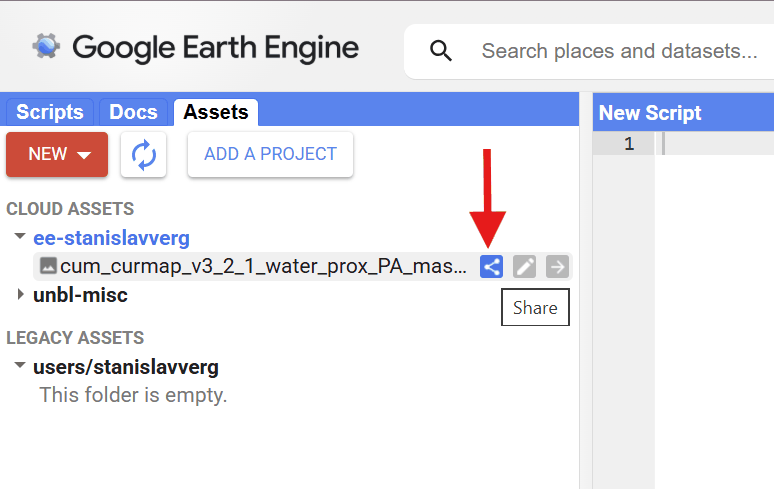
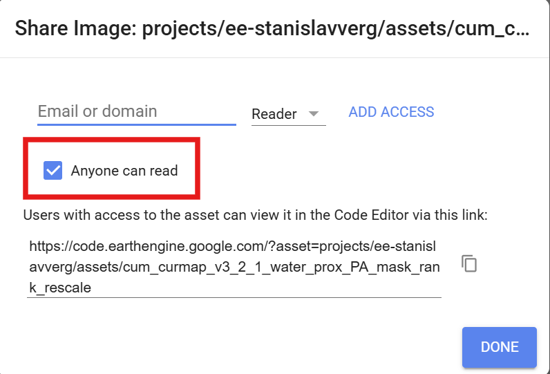
1. If you are configuring an asset from your personal Cloud Project, ensure that the ‘Anyone can read’ box is checked for this asset.

   

   Figure 7: Google Earth Engine Assets tab with an arrow pointing to the asset's Share icon

   

   Figure 8: Google Earth Engine sharing dialog with the Anyone can read box checked and highlighted

2. Navigate to the new layer page in the UNBL admin interface and fill in relevant metadata (See ‘What parameters and metadata do I fill in when creating a layer?’).

3. In the Layer Config section:

   a. Layer type: Select ‘raster’.

   b. Layer provider: Select ‘Google earth engine’.

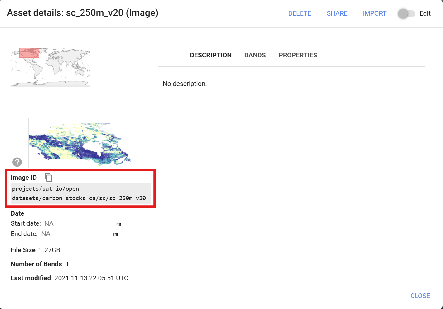
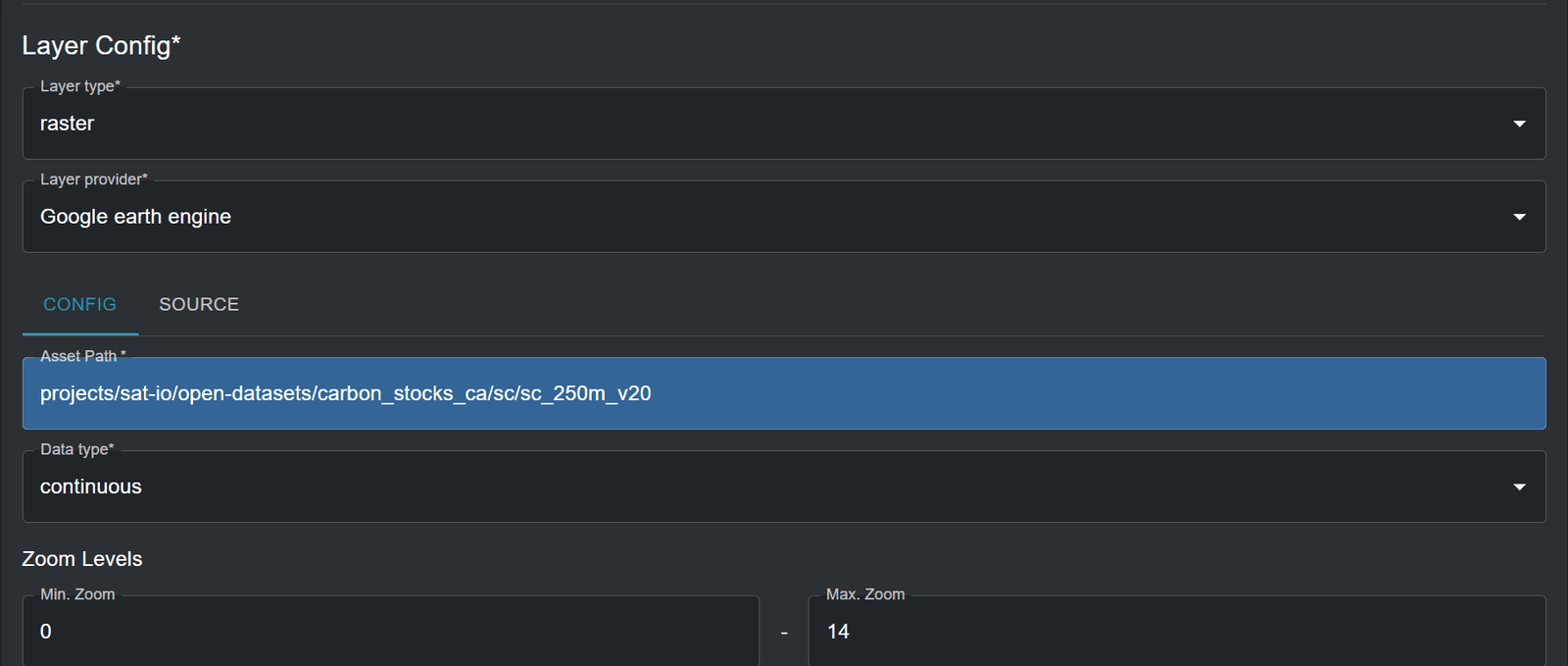
   c. Asset Path: Copy and paste the image ID of your GEE asset. Any image ID can be configured on UNBL, provided that it is a single raster band image. It can be an image ID of your personal GEE Cloud Project, or any other shared GEE Cloud Project or publicly available GEE dataset, such as one from the public catalogue awesome-gee-community-catalog, which provides access to over 4,000 public GEE assets.

   

   Figure 9: Google Earth Engine Asset details window with the Image ID highlighted

   d. Data type: Specify whether the raster image contains ‘categorical’ or ‘continuous’ data. Categorical data represents discrete classes or categories where each pixel value represents a distinct type or class. Continuous datasets represent data where values can fall anywhere within a specified range of values.

   e. Minimum/Maximum zoom level (optional): The default zoom level range is set to 0 to 14. You can optionally specify the zoom levels for the layer if the raster image only contains data at certain zoom levels. Note that UNBL supports a maximum zoom level of 14.

   

   Figure 10: Layer configuration with Google earth engine provider and the image ID pasted as Asset Path

   f. Layer styling: The layer styling determines how the legend for the GEE asset is displayed on the map, and it is also used to generate the Styled Layer Description (SLD) which influences the styling of the GEE asset in the map view. By clicking on ‘ADD ADDITIONAL STYLING’ you can specify any number of layer styling entries (also known as classes or thresholds) to match the values in the raster image. Each layer styling entry should define the following properties:

   • Value - the pixel value in the data to define the styling for.

   • Name – the name of the class or range in the layer legend on the map.

   • Color – the colour of pixels with the specified value on the map. You can define a colour through the manual colour picker, or by entering a RGBA or Hexadecimal value. Optionally, you can set the opacity of the colour in a range from 0 to 100%, where 0% is fully transparent and 100% is fully opaque.

   You can also optionally choose whether a styling entry’s name label is hidden in the layer legend on the map by clicking the

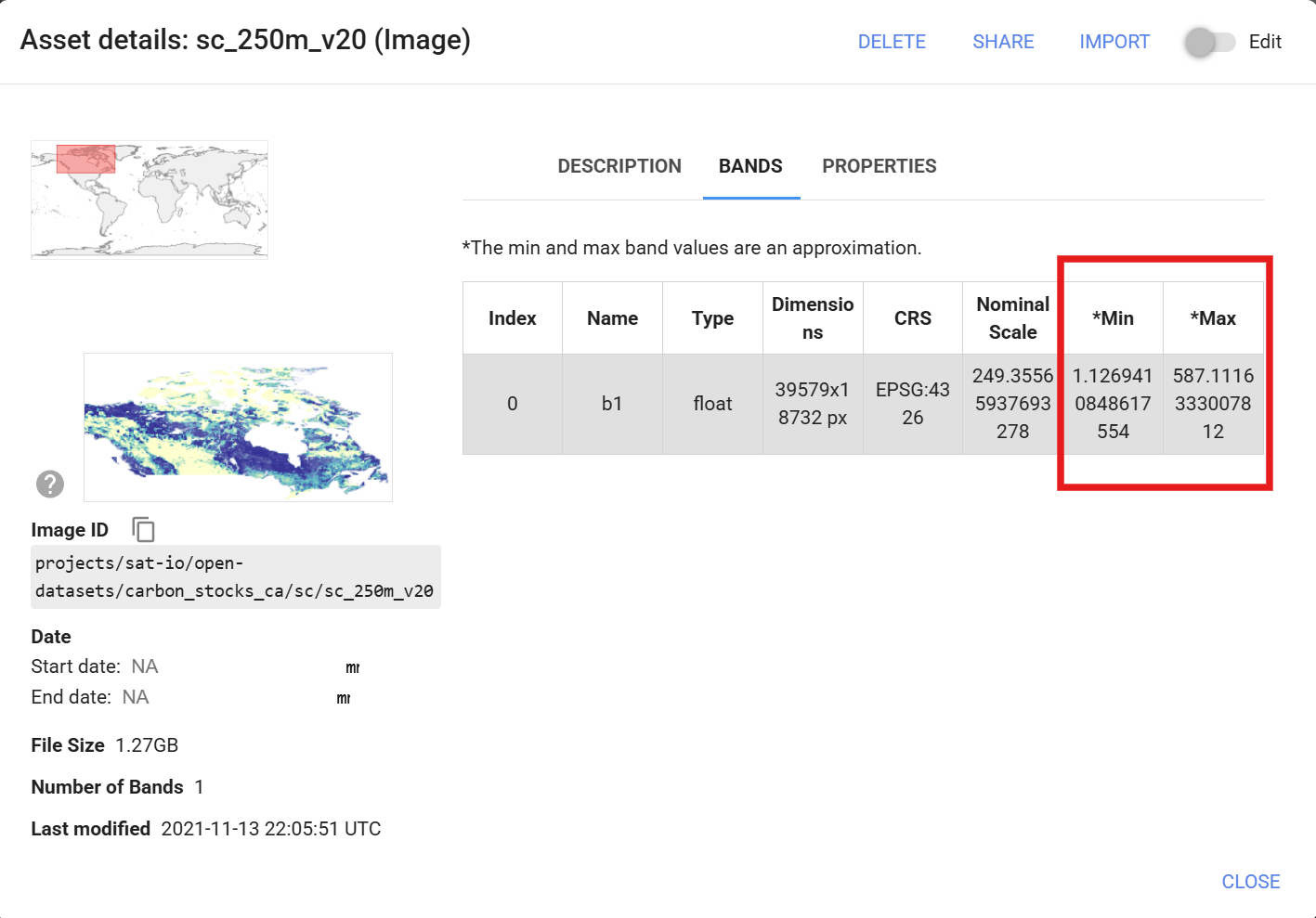
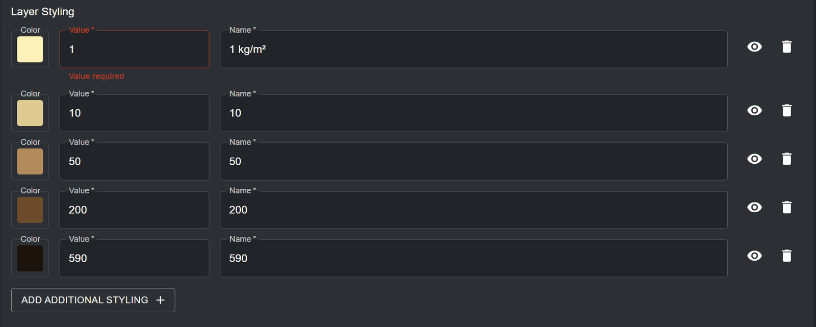
   icon next to the styling entry. For categorical layers, layer styling value entries must map to the values of each category/class within the raster data source. For continuous layers, layer styling value entries must map to the range of values within your raster file that you want rendered on the map. You can specify any points along the range of values between the minimum and maximum values -- a gradient of colours between each of these values will be generated. It is important to note that the minimum and maximum pixel values, and therefore the range of values, can be derived directly from viewing the ‘BANDS’ tab in the ‘Asset details’ information box of your asset on

   Figure 11: Visibility toggle (eye)

   GEE. The example layer styling below creates a continuous colour palette for carbon stock concentration.

   

   Figure 12: BANDS tab of the Google Earth Engine asset details with Min and Max values highlighted

   

   Figure 13: Continuous layer styling entries for carbon stock values from 1 to 590 kg/m²

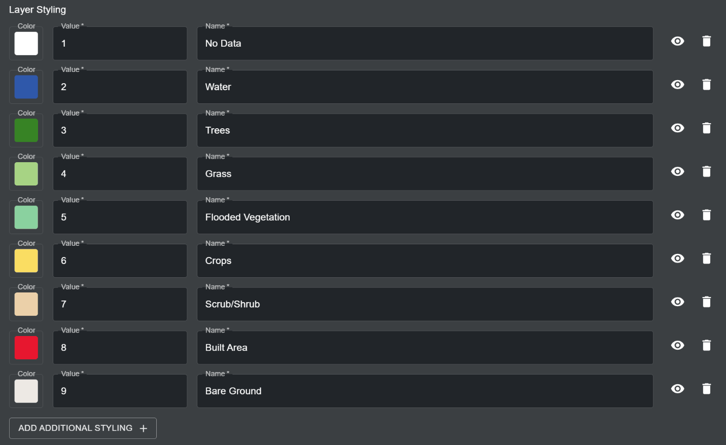
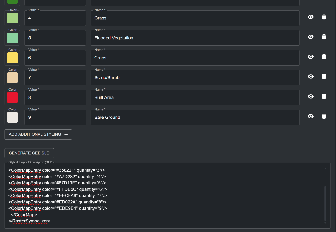
   For categorical raster layers, each specified pixel value maps to exactly one discrete class or category. The example layer styling below creates a discrete colour palette that maps land cover classes.

   

   Figure 14: Categorical layer styling entries mapping nine land cover classes to colours

   g. Styled Layer Description (SLD): Click on the ‘GENERATE GEE SLD’ button to automatically generate a SLD for configuring your GEE asset style on UNBL, based on the parameters you set for the Layer styling in step f. While layer styling determines the style of the layer legend, the SLD will determine the colour style of the actual pixels in your data. Based on the examples provided in step f, the SLD configuration for a continuous colour scheme for carbon stock concentration would look like this:

   <RasterSymbolizer>
   <ColorMap type="ramp" extended="false">
       <ColorMapEntry color="#FFF1B8" quantity="1"/>
       <ColorMapEntry color="#E2C98F" quantity="10"/>
       <ColorMapEntry color="#B58A5A" quantity="50"/>
       <ColorMapEntry color="#6E4A28" quantity="200"/>
       <ColorMapEntry color="#1C130C" quantity="590"/>
   </ColorMap>
   </RasterSymbolizer>
   

   For the categorical land cover land use raster, the SLD configuration would look like this:

   <RasterSymbolizer>
   <ColorMap type="values" extended="false">
       <ColorMapEntry color="#FFFFFF" quantity="1"/>
       <ColorMapEntry color="#1A5BAB" quantity="2"/>
       <ColorMapEntry color="#358221" quantity="3"/>
       <ColorMapEntry color="#A7D282" quantity="4"/>
       <ColorMapEntry color="#87D19E" quantity="5"/>
       <ColorMapEntry color="#FFDB5C" quantity="6"/>
       <ColorMapEntry color="#EECFA8" quantity="7"/>
       <ColorMapEntry color="#ED022A" quantity="8"/>
       <ColorMapEntry color="#EDE9E4" quantity="9"/>
   </ColorMap>
   </RasterSymbolizer>
   

   Where each ColorMapEntry colour and associated pixel quantity row matches exactly to a layer styling entry row from step f.

   

   Figure 15: Layer styling entries with the GENERATE GEE SLD button and the generated SLD code below

4. Once all metadata and configuration properties have been specified, the ‘SAVE AND VIEW DETAILS’ button will light up blue, provided that all the entered information is valid. Click on this button to configure your raster image to your workspace. See ‘How do I publish my layer and share it with external users?’ and ‘How do I edit my added layers?’ for next steps.

How do I configure raster layers using Spatiotemporal Asset Catalog (STAC)?

The STAC configuration feature is currently in testing and is subject to future updates. If you want to configure a new layer coming from an external STAC Catalogue in your UNBL workspace, please contact us at support@unbiodiversitylab.org so that we can understand the use case for this feature.

How do I configure vector layers using external tile services?

UNBL supports the configuration of vector tile layers to your workspace by linking to external tile service providers. Vector layers are discrete geometric shapes, such as points and polygons. To add geospatial data to your workspace using this method:

1. Navigate to the layer edit page and fill in relevant metadata (See ‘What parameters and metadata do I fill in when creating a layer?’).

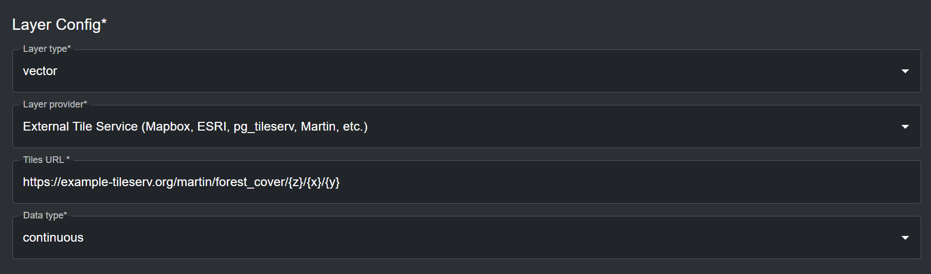
2. In the 'Layer Config' section (all fields are mandatory unless specified otherwise):

   a. Layer type: Select ‘vector’.

   b. Layer provider: Select ‘External Tile Service (Mapbox, ESRI, pg_tileserv, Martin, etc.)’.

   c. Tiles URL: Here, you can connect to an external vector tile service provider that hosts your geospatial data, such as Mapbox, ESRI, pg_tileserv, Martin, and others. To configure layers using these providers, you must supply a valid tile URL, which must contain either the placeholders {z}{x}{y} or the placeholder {bbox-epsg-3857}. For example, a configurable layer URL for a forest cover dataset hosted on Martin looks like this:

   https://example-tileserv.org/martin/forest_cover/{z}/{x}/{y}
   

   d. Data type: Specify whether the vector tiles contain ‘categorical’ or ‘continuous’ data. Categorical data represents discrete classes or categories. Continuous datasets represent data where values can fall anywhere within a specified range of values. While vector tiles can store multiple data attributes, you can only choose one data attribute for layer legend styling on UNBL. You should specify the data type based on the provisional layer legend of your added layer on UNBL.

   

   Figure 16: Vector layer configuration from an external tile service with a Martin tiles URL

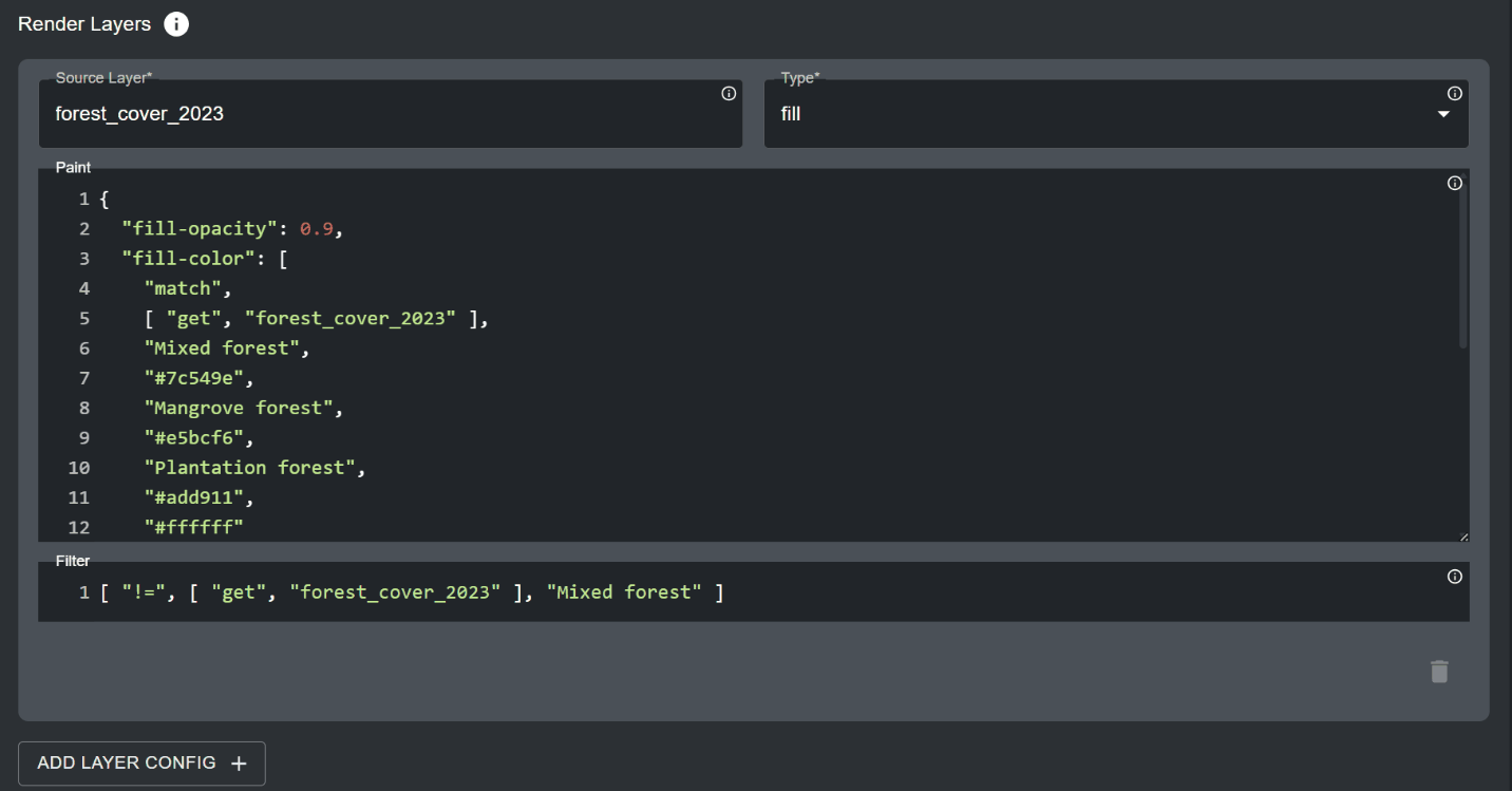
3. The ‘Render layers’ section specifies the data attributes from the vector data source that should be displayed on the map. In this section:

   a. Source layer: Specify the name of the dataset which you are hosting on the vector tile server. For example, the source layer for the example URL from step 2c is forest_cover. Click on the

   icon for this property to view detailed documentation on source layer referencing.

   Figure 17: Information

   b. Type: Specify the geometry type your dataset represents. Available options are fill, line, symbol, circle, heatmap and fill-extrusion. In the majority of cases, the geometry type will be fill (polygons with a colour fill ramp). Click on the

   icon for this property to view detailed documentation on geometry type options.

   Figure 18: Information

   c. Paint (optional): Here, you can specify the layer styling for your dataset on UNBL using a .json style configuration . Click on the

   icon for this property to view detailed documentation for configuring layer styling. For the most common geometry types of type

   Figure 19: Information

   fill, the paint configuration follows a set template. For configuring layer styling for categorical datasets, use the following template:

   {
   "fill-opacity": 0.9,
   "fill-color": [
   "match",
   [ "get", "forest_cover_2023" ],
   "Mixed forest",
   "#7c549e",
   "Mangrove forest",
   "#e5bcf6",
   "Plantation forest",
   "#add911",
   "#ffffff"], 
   "fill-outline-color": [ 
   "match", 
   [ "get", "forest_cover_2023" ], 
   "Mixed forest",
   "#7c549e",
   "Mangrove forest",
   "#e5bcf6",
   "Plantation forest",
   "#add911",
   "#ffffff" ]
   }
   

   The same template, in text format below, highlights strings which are configurable variables and need to be changed based on your layer styling:

   { "fill-opacity": 0.9, "fill-color": [ "match", [ "get", "forest_cover_2023"], "Mixed forest", "#7c549e", "Mangrove forest", "#e5bcf6", "Plantation forest", "#add911", "#ffffff"], "fill-outline-color": [ "match", ["get", "forest_cover_2023"], "Mixed forest", "#7c549e", "Mangrove forest", "#e5bcf6", "Plantation forest", "#add911", "#ffffff"] }

   where:

   • fill-opacity sets the opacity of the polygon fill, from 0 (fully transparent) to 1 (fully opaque).

   • fill-color specifies the data attribute which will be used to style the polygon fill, as well as the styling itself (in this instance, it is the forest_cover_2023 attribute of the forest_cover example source dataset mentioned earlier, and match specifies styling for discrete categories for this data attribute). Each next configurable text string pair specifies a discrete category of your data attribute and the colour you want to paint that specific category (in Hex code format), respectively.

   • fill-outline-color functions the same as fill-color, but specifies the colour of the linear boundary of the polygon instead of the inner polygon fill. This way, you can specify a different colour boundary for polygons compared to the colour of their inner fill (note that this is not the case for the above example). Importantly, you can specify a “#ffffff” string at the end of the last hex code string for either of the fill properties to signify that any data categories which are not explicitly listed in the fill styling property should be transparent.

   Important

   If you do not include the “#ffffff” string for transparent styling for non-included data categories, your vector tiles will fail to visualize if you fail to exhaustively specify styling for all data categories that are present in your data attribute in the fill styling property. However, you do not have to specify inclusive transparent styling if you specify a filter to exclude selected data categories in your data attribute from consideration for layer styling (step 3d).

   For configuring layer styling for continuous datasets, use the following template:

   {
   "fill-opacity": 0.9,
   "fill-color": [
   "interpolate",
   [ "linear" ],
   [ "get", "canopy_height_2023" ],
   0, 
   "#f5ebd5", 
   5, 
   "#eef5c9", 
   10, 
   "#dbe6a1", 
   20, 
   "#c5e897", 
   30, 
   "#9fe04a", 
   50, 
   "#689c24", 
   75, 
   "#518510", 
   100, 
   "#305207" ], 
   "fill-outline-color": [
   "interpolate",
   [ "linear" ],
   [ "get", "canopy_height_2023" ],
   0, 
   "#f5ebd5", 
   5, 
   "#eef5c9", 
   10, 
   "#dbe6a1", 
   20, 
   "#c5e897", 
   30, 
   "#9fe04a", 
   50, 
   "#689c24", 
   75, 
   "#518510", 
   100, 
   "#305207" ]
   }
   

   The same template, in text format below, highlights strings which are configurable variables and need to be changed based on your layer styling:

   { "fill-opacity": 0.9, "fill-color": [ "interpolate", [ "linear" ], [ "get", "canopy_height_2023" ], 0, "#f5ebd5", 5, "#eef5c9", 10, "#dbe6a1", 20, "#c5e897", 30, "#9fe04a", 50, "#689c24", 75, "#518510", 100, "#305207" ], "fill-outline-color": [ "interpolate", [ "linear" ], [ "get", "canopy_height_2023" ], 0, "#f5ebd5", 5, "#eef5c9", 10, "#dbe6a1", 20, "#c5e897", 30, "#9fe04a", 50, "#689c24", 75, "#518510", 100, "#305207" ] }

   where:

   • fill-opacity sets the opacity of the polygon fill, from 0 (fully transparent) to 1 (fully opaque).

   • fill-color specifies the data attribute which will be used to style the polygon fill, as well as the styling itself (in this instance, it is the canopy_height_2023 attribute of the forest_cover example source dataset mentioned earlier, and interpolate specifies styling for a continuous range of values for this data attribute). Each next configurable variable pair specifies a number that falls within the range of values in your data attribute and a text string with the colour you want to paint that specific value (in Hex code format), respectively. To build a continuous colour scheme for your data attribute, start by styling the minimum value and work upwards in reasonable intervals, based on the spread of your data, to reach the maximum value. Any values falling between a specified interval will be styled using a graduated colour that is darker than the smaller value specified colour, and lighter than the larger value specified colour in the specified interval.

   • fill-outline-color functions the same as fill-color, but specifies the colour of the linear boundary of the polygon instead of the inner polygon fill. This way, you can specify a different colour boundary for polygons compared to the colour of their inner fill (note that this is not the case for the above example).

   d. Filter (optional): You can optionally specify a subset of data categories, or specific range of values, which should be used for styling the map. Any data categories or range of values falling outside of the specified filter will not be considered in the layer styling. Click on the

   icon for this property to view detailed documentation for configuring filter options. As an example, if you wanted to filter out the “Mixed forest” category from the

   Figure 20: Information

   forest_cover_2023 data attribute, you would use the following template:

   ["!=", ["get", "forest_cover_2023"], "Mixed forest"]
   

   where != specifies a conditional exclusion expression.

   

   Figure 21: Render Layers section with source layer, fill type, paint expression and filter

   e. ADD LAYER CONFIG (optional): In some cases, you may wish to configure styling for more than one data attribute in your vector dataset. By clicking on this button, you can specify further styling expressions. Note that any data attributes, data categories or value ranges that overlap between styling expressions or are contained within the same polygons in your data and are not filtered out accordingly, will lead to a confusing layer visualization.

4. The 'Interaction config' section specifies the data attributes in the vector dataset that should be displayed in the popup when clicking on the vector layer's polygons on the map. Click on ‘ADD ADDITIONAL OPTION’ to specify a data attribute that should be displayed in the popup. This is an optional section – it can be left blank if unneeded. For each Interaction config entry:

   a. Column: The name of the data attribute which will be displayed (case sensitive). For example, for the forest_cover source layer, the data attribute could be forest_cover_2023 or canopy_height_2023.

   b. Type: Choose string, date or number type, depending on the format of your data attribute.

   c. Format (optional): If your data attribute is of date or number type, you can specify the formatting here (e.g. dd/mm/yyyy for date).

   d. Property (optional): Here, you can specify the label of the data attribute displayed in the popup table.

   e. Prefix (optional): You can specify a prefix that will be displayed in front of the data attribute’s value/category. Note that this will be displayed after the property label.

   f. Suffix (optional): You can specify a suffix that will be displayed after the data attribute’s value/category (e.g. units).

   g. Click on the

   icon to remove an Interaction config entry.

   Figure 22: Delete (bin)

   

   Figure 23: Interaction config entries for forest type and canopy height attributes

   

   Figure 24: Map pop-up showing attribute values after clicking a vector layer polygon

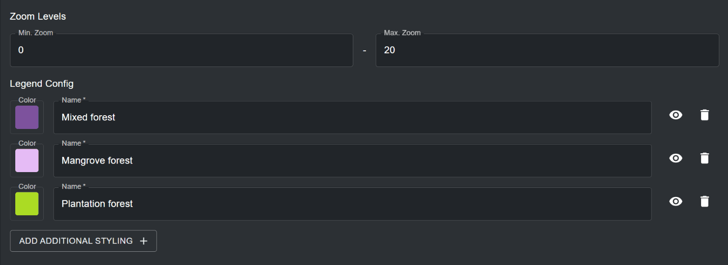
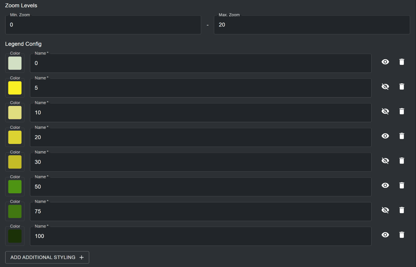
5. Specify the zoom levels for your vector tiles. The default zoom level range is set to 0 to 20. You can optionally specify the zoom levels for the layer if the vector tiles are only viewable at a smaller/larger resolution. Note that UNBL supports a maximum zoom level of 20 for vector tiles.

6. Specify the legend styling for your vector tile layer in the 'Legend Config' section. In this section (all fields are mandatory unless specified otherwise):

   a. By clicking on ‘ADD ADDITIONAL STYLING’ you can specify any number of layer styling entries to match the data categories/range of values in your vector tile layer. Each layer styling entry should define the following properties:

   • Name – the name of the styling entry in the layer legend on the map.

   • Color – the colour associated with the specified name in the layer legend. You can select a colour by using the colour picker, or by specifying a RGBA or Hex colour code value.

   You can also optionally choose whether a styling entry’s name label is hidden in the layer legend on the map by clicking the

   icon next to the styling entry. For categorical data, the legend layer styling entries should represent the discrete categories and their associated colour styling which you specified in the 'Render layers' section. For continuous data, legend styling entries should represent the range of values and their associated colour gradient which you specified in the 'Render layers' section.

   Figure 25: Visibility toggle (eye)

   

   Figure 26: Vector layer zoom levels and legend config with three forest categories

   

   Figure 27: Legend config for continuous vector data with some entry labels hidden from the legend

7. Once all metadata and configuration properties have been specified, the ‘SAVE AND VIEW DETAILS’ button will light up blue, provided that all the entered information is valid. Click on this button to configure your vector tile layer to your workspace. See ‘How do I publish my layer and share it with external users?’ and ‘How do I edit my added layers?’ for next steps.

How do I publish my layer and share it with external users?

To make any of your added layers discoverable and viewable to all users of your workspace (see ‘How do I view datasets within my workspace?’, as well as optionally make your layer viewable to users outside of your workspace, undertake the following steps:

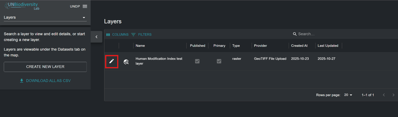
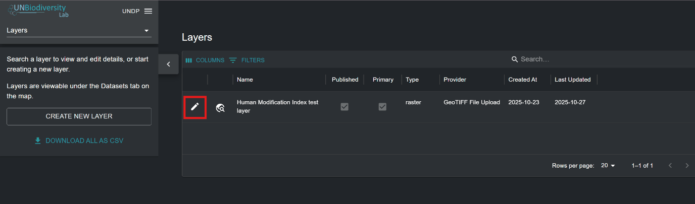
1. Navigate to the edit layer page for your layer of choice. Upon adding a layer to your workspace, you will be automatically taken to this page. Alternatively, click on the

   button in the layer list available after navigating to the ‘Layers’ page in your admin interface.

   Figure 28: Edit (pencil)

   

   Figure 29: Layers page list with the edit button for a layer highlighted

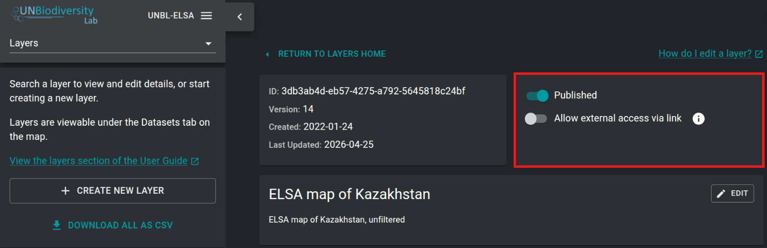
2. For your dataset to be accessible in the UNBL map view, you must publish the dataset by clicking the ‘Published’ toggle button. Unpublished datasets remain in the admin interface until you are ready to publish them to the UNBL map view.

3. If your dataset is published, a toggle button will appear with an option to ‘Allow external access via link’. This is an optional toggle that, if enabled, makes your layer accessible to anyone with the map view URL, even users outside your workspace. To share your layer URL, copy the link that appears or click on the

   icon to copy the link automatically to your clipboard.

   Figure 30: Copy

4. You don't need to mark layers as primary: UNBL does this automatically. A layer that is not part of a group layer is primary, so it appears as its own entry in the ‘DATASETS’ search bar on UNBL. A layer that is part of a group layer is not primary, and is found through its group layer instead (see ‘How do I create group layers?’). The layer list in your admin interface shows each layer's ‘Primary’ status for information only.

   

   Figure 31: Edit layer page with the Published and Allow external access via link toggles highlighted

How do I edit my added layers?

You may want to go back and edit your added layers to change any of the associated metadata, test if your layer is visualizing on UNBL, and edit your layer configuration accordingly if your layer is not visualizing. To do this:

1. Navigate to the edit layer page for your layer of choice. Upon adding a layer to your workspace, you will be automatically taken to this page. Alternatively, click on the

   button in the layer list available after navigating to the ‘Layers’ page in your admin interface.

   Figure 32: Edit (pencil)

   

   Figure 33: Layers page list with the edit button for a layer highlighted

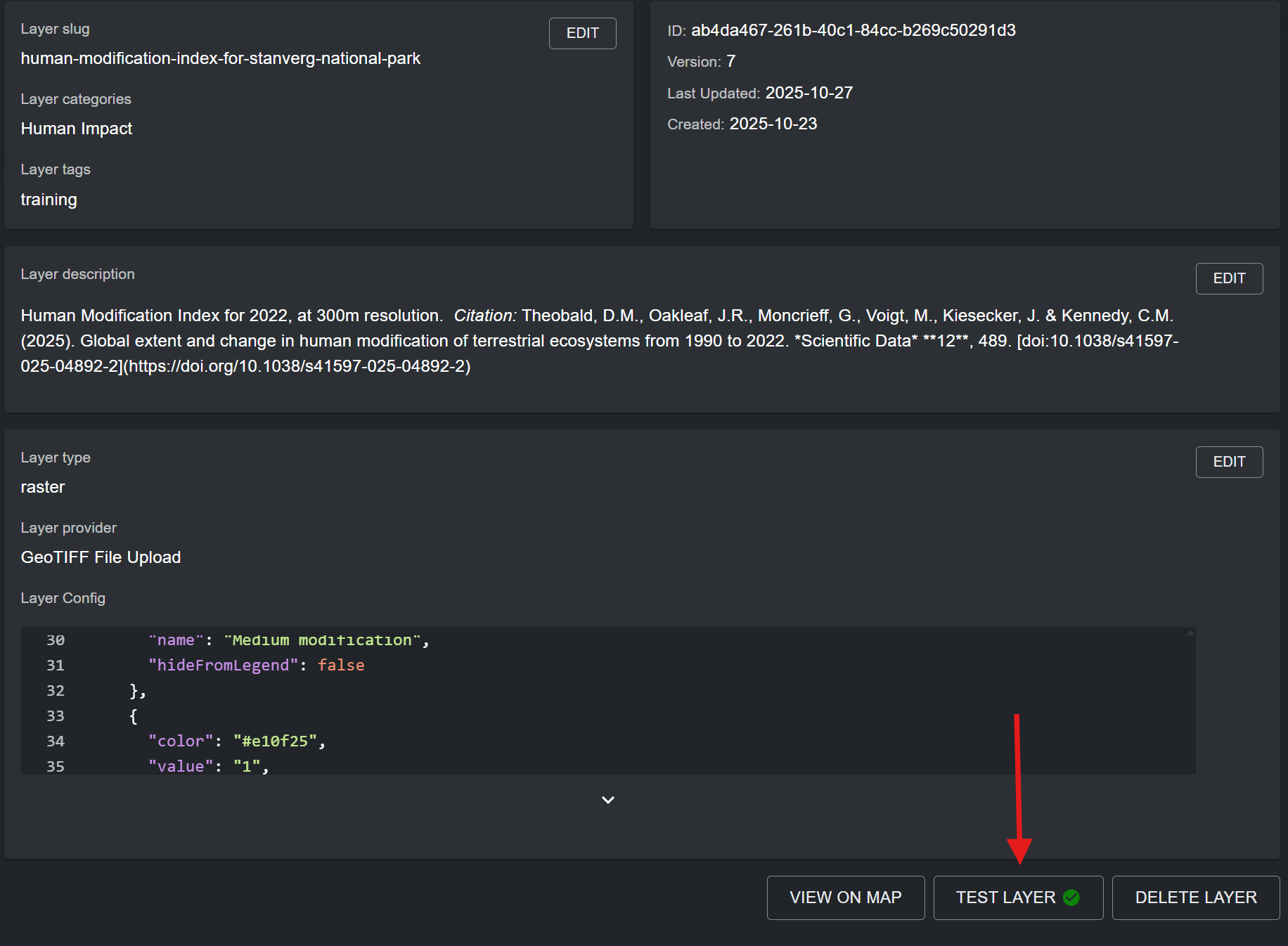
2. To test if your layer is visualizing properly in the UNBL map view, click on the ‘TEST LAYER’ button in the bottom right corner of the edit layer page. A green tick will appear inside the button if the layer has been correctly uploaded and/or configured. Otherwise, a red cross will appear with an error message diagnosing the problem.

   Note

   If you are uploading a regional dataset (non-global extent), it is possible that the test may report a failure even if the layer is working, as the test may request sample tiles that fall outside of your dataset’s areal extent. Alternatively, the test may report a positive result solely due to a valid external layer URL, even if the layer is failing to visualize in the map view due to an incorrect layer styling configuration. Therefore, it is always best practice to double check the test layer diagnosis by verifying manually whether your layer is visualizing in the UNBL map view.

   

   Figure 34: Edit layer page with arrow pointing to TEST LAYER button showing a green tick

3. If you want to navigate directly to your layer in the UNBL map view, click on the ‘VIEW ON MAP’ button. If you want to delete your layer from your workspace, click on the ‘DELETE LAYER’ button.

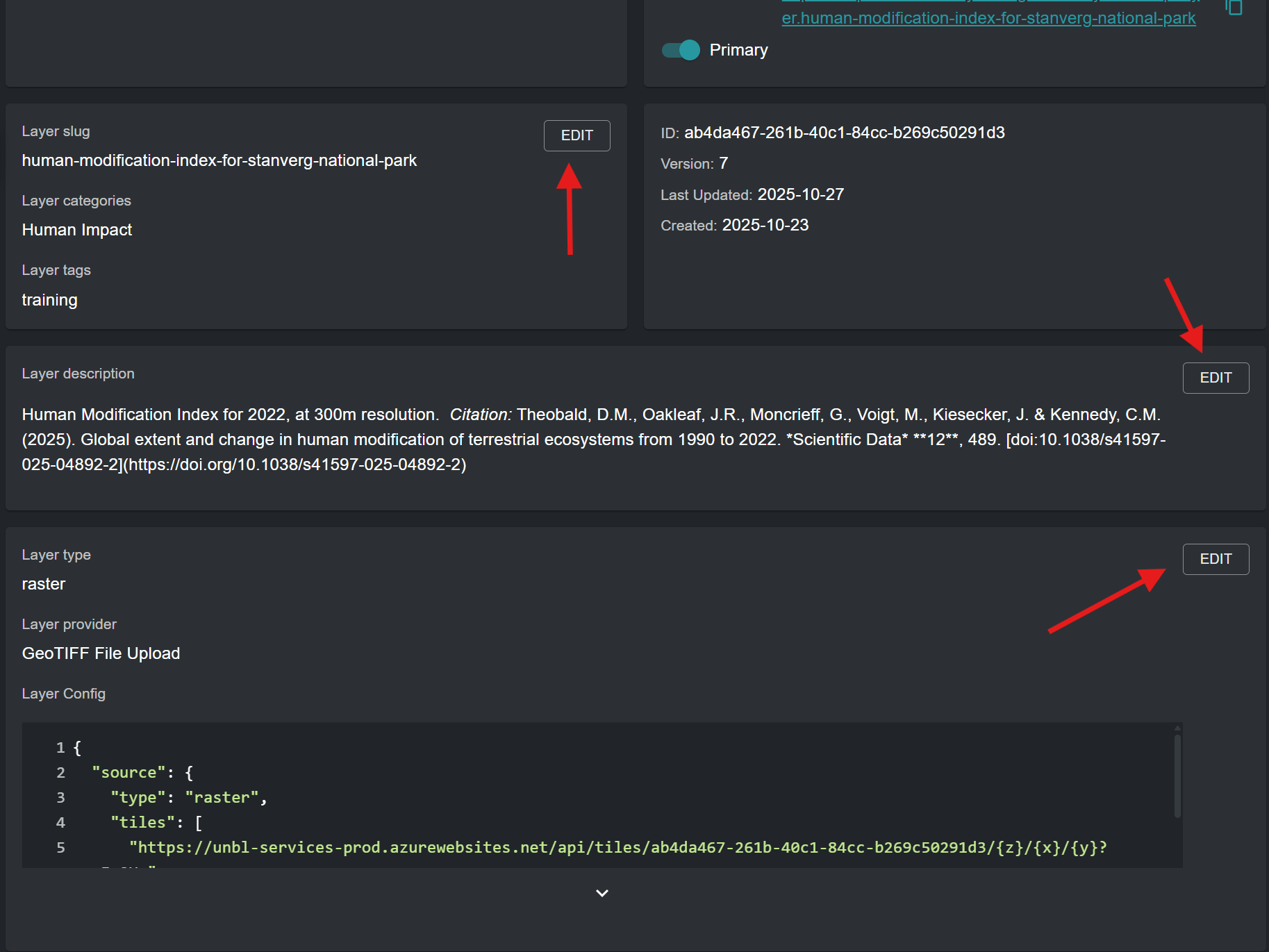
4. Click on the ‘EDIT’ button for any of the layer metadata/configuration sections to edit information and parameters for that section.

   

   Figure 35: Edit layer page with arrows pointing to the EDIT buttons of each section

How do I create group layers?

Any layers that you add to your UNBL workspace can be grouped together to organize multi-year or multi-categorical data. Each year or category is akin to an individual raster band. Group layers are created in a new, separate layer (termed parent layer on UNBL) to the component layers (termed child layers on UNBL). For example, a land cover raster spanning three years would require four layers to be made: each year as its own child layer, as well as a fourth parent layer they will all be accessible from. In this case, each child layer must be published. Because they belong to a group layer, UNBL automatically treats the child layers as not primary, so they are found in the map view through the group layer rather than as separate entries. The group/parent layer is an additional display layer with a fixed layer configuration which references all child layers. It must also be published. When the group layer is viewed on UNBL, a single layer legend appears from which you can select any one of your included child layers to be visualized in the map view.

Note

Child layers inherit metadata from their group layer. In the map view, a child layer's information shows the group layer's description first, followed by the child layer's own description. All other metadata fields (sources, citation, licence, disclaimer, read more links, download links, resolution, data version, start date, end date and publication date) use the child layer's own value if it has one, and otherwise the group layer's value. So fill in shared information once, on the group layer, and add to a child layer only what is specific to it. A field left blank, including a date with every part cleared, counts as not set, and the child layer then takes the group layer's value.

To set up a group layer:

1. Publish all child layers to be included in the group layer. The public URL feature works in the same way as for standalone layers (see ‘How do I publish my layer and share it with external users?’).

2. Create a separate layer using the ‘CREATE NEW LAYER’ button in the ‘Layers’ page of the admin interface for your workspace. This will be your designated group layer.

3. Enter a layer title, layer slug, layer category, search tag, and a layer description which is representative of the dataset represented by your collection of child layers. The group layer's description, sources, citation and other metadata are shown for all of its child layers (see the note above), so fill in here everything that applies to the whole collection. For more information on filling in metadata for layers, see ‘What parameters and metadata do I fill in when creating a layer?’.

4. Layer type: Select ‘group’.

5. Grouped layers: From the dropdown menu, select all child layers which you want to include in your group layer. Available layers for inclusion are all added layers in your workspace.

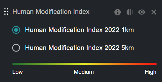
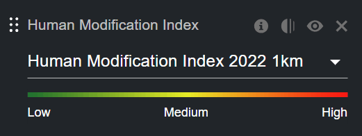
6. Layer selector: From the dropdown menu, select either ‘Dropdown’ or ‘Radio Button’. These options influence how the layer selector UI appears in the layer legend of the group layer on UNBL. The dropdown option is recommended for group layers with more than three child layers. The radio button option is recommended for group layers with three or less child layers, or when group layers represent the same data with different styling.

   

   Figure 36: Group layer legend on the map with a radio button layer selector

   

   Figure 37: Group layer legend on the map with a dropdown layer selector

7. Click the ‘SAVE AND VIEW DETAILS’ button to add the group layer to your workspace.